It will come to no surprise to any one of my friends that I am easily nerdsniped. Sometimes, it takes just a small unusual thing to capture my attention and turn my next weekend into the most unproductive (but fun) black hole of time. One of those moments arose this summer when Benjamin, my beloved potted ficus tree, found himself to be the breeding ground of a particularly productive fungus gnat. That little bug must have laid hundreds of eggs into Benjamin's soil, and somehow orchestrated all of his little sons and daughters to hatch on the same particularly beautiful Thursday morning.
Right after waking up, I saw hundreds of little gnats whizzing around in my living room. Luckily, I still had some sticky fly traps lying around. I placed half of them into Benjamin's soil and the other half high on the wall near the window, where most of the little gnats seemed to concentrate. When I returned from work later that day, I was caught off guard. The traps in Benjamin's soil were expectedly quite packed already, but when I looked at the traps near the ceiling, I had to pause for a second.
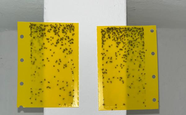
That can't be random, can it?
Am I crazy for seeing a pattern here? I knew the little bugs often flew closer to the ceiling, but this looked almost like a gradient. But no. There's no way I would spend my weekend trying to investigate the pattern of flies on a sticky trap, right?
Well... you're reading this post, so I guess my monkey mind won that fight. Where there is a pattern, there's a project.
Two birds flies with one stone
I have been wanting to learn some basic computer vision (CV) for a while anyway, so when life decided to give me hundreds of little black lemons, I assumed I should make a delicious CV lemonade. My plan was as simple as it was unclear:
- use CV magic to identify the flies
- plot the frequency of flies against their distance to the ceiling
- see if there is actually a pattern
stop and be happy- improvise from here
Since I had zero experience in CV, I googled my way through some tutorials of object recognition with OpenCV. Starting out seemed straightforward: I applied some manual adjustments to my photo (crop, desaturate, increase constrast) in order to clearly separate the little points from the background and to make subsequent steps easier. This was also the point where I realised that my (now) scientific experiment would have been quite a lot more scientific if I had mounted the fly traps at the exact same height and taken a photo from a perfectly straight perspective. In reality, I took a quick snapshot to send to a friend and then threw them away. I guess this is what you get for not thoroughly planning your pest control with subsequent data analysis in mind.
I loaded up OpenCV and found that it has a findContours method already - neat! After some fine-tuning of the parameters and applying a small clustering kernel, I found a result that looked promising. The next step then was to find the center of each contour (more OpenCV magic) and to do a small visual comparison. Here is the result:
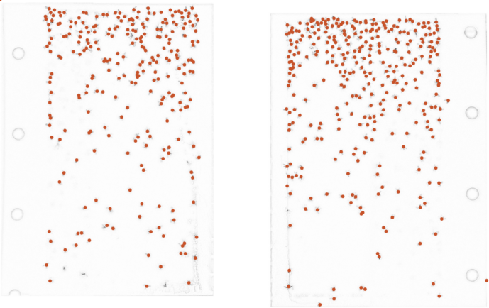
Gnat detection. You can find the code in the appendix.
All in all, the algorithm detected everything almost perfectly. That's step one done! With the x/y coordinates available through the center points, step two was as easy as binning the height of all points into height buckets and plotting the result.
I looked at the output and was positively surprised:
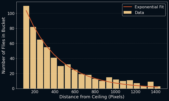
Very exponential indeed! (Code available in the appendix.)
That does look quite regular. As you can see, I also created an exponential fit with scipy's curve_fit function, which fits the data surprisingly well. So that's it then? Gnats fly closer to the ceiling in a seemingly exponential fashion. That's a fun conclusion to this little adventure. Right, monkey brain? Back to some real work, right?
...right?
Sigh. But why should they form an exponential curve? Is it actually exponential? I guess I could have also fit a quadratic curve and found a similarly nice looking plot. After all, to quote Johnny von Neumann: With four parameters I can fit an elephant, and with five I can make him wiggle his trunk. So is there any research about the flight patterns of fungus gnats? Are there gnat-experts? (Gnatsperts?) A quick google search surfaced A Review of the Scientific Literature on Fungus Gnats from 1996. Cytogenetics... Taxonomy... Life History... Economic importance. Huh. "Fungus gnats are weak flyers, but very active and rapid runners". They must not have seen my breed then. More quick googling did not reveal much else (except that house flies can reach heights of up to 1800 meters / 5900 ft on hot days. A quick re-measure later I was confident that my ceiling was lower than that). So why the gradient? There was no wind in my room, and the temperature gradient across a few centimeters surely must be negligible, right? Do my little friends just have an inherent bias towards flying up?
When all you have is a hammer...
I didn't have any answers, but I could test that last thesis somewhat. I like simulations, and when all you have is a hammer, even fly patterns can look like very suitable nails. To simulate a fly-infested room, I put dozens of virtual flies into a 100 by 100 pixel box and defined a few basic rules:
- each fly starts at a random x/y coordinate, with a random speed v_x/v_y in each direction
- after random time intervals, each fly randomly flies in a new direction with a new random v_x/v_y
- whenever a fly hits a wall, it gets reflected back in the opposite direction
Now, this would of course just result in random movement (Brownian motion). So let's add one rule that I call the "law of instinct" (because I can't explain why it should exist from first principles, and naming it makes it seem like I still know what I'm doing):
- because every fly is afraid of the evil fly-eating animals on the ground, it has a tiny upwards-bias in its y-speed every time it randomly chooses a new v_y
Let's see what happens when I run the simulation. I also added the fly-count bins at each time step on the right to see how the distribution changes over time. The axes are flipped here to match the simulation.
Fly, you fools!
That does look quite similar to my distribution. That's a good start. To find out which pattern my simulated friends formed after settling in, I calculated the average number of flies in each bin over the final 200 simulation steps and used the same fit approach as before to put an exponential curve on top of it.
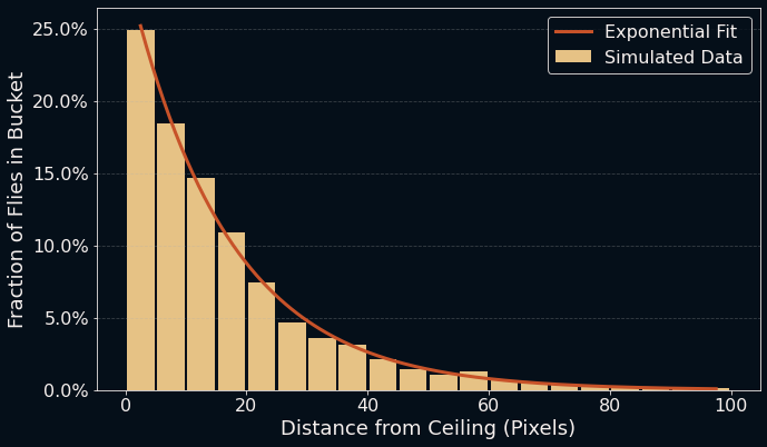
Yes, it would have been more obvious to linearise the data, but who likes log-scales? Crazy people and lumberjacks, that's who.
So yes. Exponential again, this time quite clearly so. Of course, this was a simulation with my own arbitrary rules that have no basis in reality, so I couldn't draw any conclusions from it. But at least I had some fun animations now that I could look at. The tiny simu-flies look a bit like small gas molecules zipping around in a container. I guess they could, in some way, be seen as similar. Hmm... what would it look like if my flies were tiny molecules governed by the Navier-Stokes equations, guided towards the ceiling by some tiny natural force? If I described them that way, couldn't I find an analytical answer to the question of their distribution?
Somewhere, some place deep inside my head, I could feel a tiny monkey smiling.
...sigh.
Gaseous flylecules
Allright. Let's try to get this done quickly.
Starting from the Navier-Stokes equation for momentum, ρ(∂u/∂t+u∇u)=−∇p+∇⋅τ+ρg, and assuming steady state with no movement (u=0) and no pressure gradients in the other axes (so ∇p=dp/dy), you can ignore most terms and land at the hydrostatic equilibrium equation with dp/dy = ρg. The change in pressure of a gas over the height is equal to the local density and its acceleration in the force field.
If we assume a constant tiny acceleration a upwards (in the direction of -y, where y is the distance from the ceiling) and ideal gas law behaviour with p = ρRT, this equation yields 1/ρ dρ = a/RT dy, which can be integrated to give an expression for ρ(y): ρ(y) = exp(-ya/RT).
So the density, again, increases exponentially towards the wall. I guess that settles... something?
But then again, isn't the constant velocity drift in my simulation something completely different from a constant acceleration in these equations? I could... you know what? No. The monkey can't always win. This is it, it's 2 AM and I need to sleep.
Conclusions
I don't know what I expected, and I'm sure I made several mistakes in my analysis, but it was a fun way to get my mind off the gnat infestation. The little flying dots are gone now, after a long battle that included me moving Benjamin into the attic for a few days, where temperatures reach approximately 7000 degrees in the summer. It's strange that that helped, since the research papers kept talking about how they are a plague in greenhouses. Why does this only lead to more questions? Oh well.
If you or anyone you know is a gnat-expert, please reach out to me. I still want to know the correct answer to this behaviour. Until then, I'm enjoying the thought of Benjamin's relief now that he is crawl-free.
Code
Code one (OpenCV for finding clusters):
def count_black_clusters(image_path, plot=True, save_path='./contours.png'):
    # Load the image
    image = cv2.imread(image_path, cv2.IMREAD_GRAYSCALE)
    if image is None:
        print(f"Error loading {image_path}")
        return None

    # turn into binary b/w
    _, binary = cv2.threshold(image, 100, 255, cv2.THRESH_BINARY_INV)

    # cluster close-by pixels
    kernel = np.ones((4, 4), np.uint8)
    closed = cv2.morphologyEx(binary, cv2.MORPH_CLOSE, kernel)

    # find contours
    contours, _ = cv2.findContours(closed, cv2.RETR_EXTERNAL, cv2.CHAIN_APPROX_SIMPLE)

    # filter contours based on min_size
    min_size = 3
    filtered_contours = [contour for contour in contours if cv2.boundingRect(contour)[2] > min_size or cv2.boundingRect(contour)[3] > min_size]

    count_clusters = len(filtered_contours)
    print(f"Number of detected clusters: {count_clusters}")

    # draw contours on image
    output_image = cv2.cvtColor(image, cv2.COLOR_GRAY2BGR)
    for contour in filtered_contours:
        # calculate the moments of each contour and find the X/Y center of mass from it
        M = cv2.moments(contour)
        if M["m00"] != 0:
            cX = int(M["m10"] / M["m00"])
            cY = int(M["m01"] / M["m00"])
        else:
            cX, cY = 0, 0

        # draw center of mass as a circle
        cv2.circle(output_image, (cX, cY), 8, [255*c for c in cmap0[0]], -1)

    if plot:
        show_and_save_image(output_image, save_path, cmap=None)

    return filtered_contours, count_clusters
Code two (bucketing and plotting):
def analyze_height_frequency(filtered_contours, num_bins=20, skip=0):
    """
    Analyzes the vertical distribution of contours and returns binned data.
    """
    frequency = np.zeros(num_bins)

    xy_dots = [[],[]]
    for contour in filtered_contours:
        M = cv2.moments(contour)
        if M["m00"] != 0:
            # Skip the top N pixels, since only one of the two fly traps has data for those
            cY = int(M["m01"] / M["m00"])
            if cY > skip:
                xy_dots[0].append(int(M["m10"] / M["m00"]))
                xy_dots[1].append(cY)

    if not xy_dots[1]: # Handle case with no contours found
        print("Warning: No contours found after skipping. Returning empty data.")
        return [np.array([]), np.array([])]

    bin_edges = np.linspace(min(xy_dots[1]), max(xy_dots[1]), num_bins + 1)
    bin_midways = [np.mean([bin_edges[i], bin_edges[i+1]]) for i in range(len(bin_edges)-1)]

    # count the numbers in each bin
    frequency, _ = np.histogram(xy_dots[1], bins=bin_edges)

    return [bin_midways, frequency]